Keras time series prediction with CNN+LSTM model and TimeDistributed layer wrapper
Keras time series prediction with CNN+LSTM model and TimeDistributed layer wrapper
I have several data files of human activity recognition data consisting of time-ordered rows of recorded raw samples. Each row has 8 columns of EMG sensor data and 1 corresponding column of target ...
stackoverflow.com
CNN + LSTM 아키텍쳐 구조
- 전반적인 CNN+LSTM 아키텍쳐를 참고하기 위해 구글링해서 첨부하였음.
- (본문 하단에 첨부한 CNN 및 데이터 구조랑 상이함)

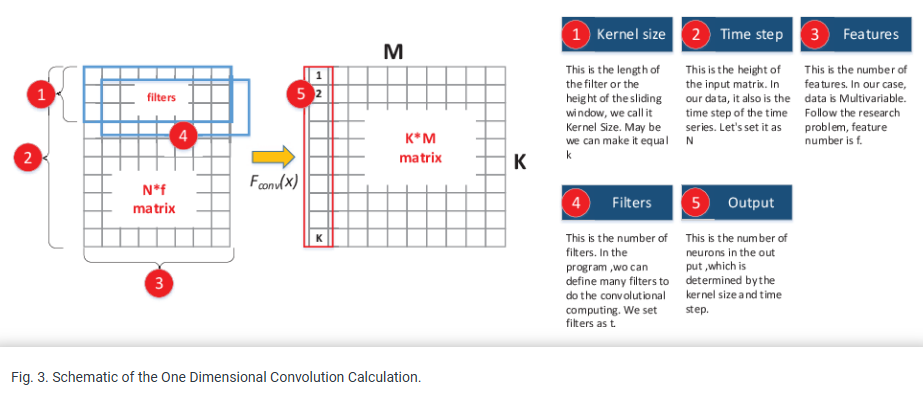
CNN + LSTM (Multivariate TimeSeries)
사용자는 인간 활동 인식 데이터를 다룬 여러 데이터 파일을 가지고 있습니다. 이 데이터는 시간 순서대로 기록된 raw 샘플 행으로 구성되어 있으며, 각 행은 8개의 EMG(근전도) 센서 데이터 열과 1개의 타겟 센서 데이터 열로 이루어져 있습니다. 사용자는 8개의 EMG 센서 데이터를 CNN+LSTM 딥러닝 모델에 입력하여 1개의 타겟 데이터를 예측하려고 합니다.
이를 위해, 데이터셋을 다음 단계로 처리합니다:
- 데이터셋 분할
데이터셋(a)을 50개의 행으로 된 윈도우(b)로 분할합니다. 각 윈도우는 연속적인 raw 샘플을 포함합니다. - LSTM 입력 데이터 구성
50행으로 나눈 윈도우 4개를 묶어 LSTM 모델의 시간 단계(time steps)로 사용합니다(c). 결과적으로, CNN+LSTM 모델의 입력은 4개의 시간 단계(윈도우)로 구성된 블록으로 형성됩니다.
 from keras.models import Sequential
    from keras.layers import CuDNNLSTM
    from keras.layers.convolutional import Conv2D
    from keras.layers.core import Dense, Dropout
    from keras.layers import Flatten
    from keras.layers import TimeDistributed

    #Code that reads in file data and shapes it into 4-window blocks omitted. That code produces the following arrays:
    #x_train  - shape of (808, 4, 50, 8) which equates to (samples, time steps, window length, number of channels)
    #x_valid  - shape of (223, 4, 50, 8) which equates to the same as x_train
    #y_train  - shape of (808, 50, 1) which equates to (samples, window length, number of target channels)


    # Followed machine learning mastery style for ease of reading
    numSteps = x_train.shape[1]
    windowLength = x_train.shape[2]
    numChannels = x_train.shape[3]
    numOutputs = 1

    # Reshape x data for use with TimeDistributed wrapper, adding extra dimension at the end
    x_train = x_train.reshape(x_train.shape[0], numSteps, windowLength, numChannels, 1)
    x_valid = x_valid.reshape(x_valid.shape[0], numSteps, windowLength, numChannels, 1)


    # Build model
    model = Sequential()
    model.add(TimeDistributed(Conv2D(64, (3,3), activation=activation, name="Conv2D_1"),
                                     input_shape=(numSteps, windowLength, numChannels, 1)))

    model.add(TimeDistributed(Conv2D(64, (3,3), activation=activation, name="Conv2D_2")))
    model.add(Dropout(0.4, name="CNN_Drop_01"))

    # Flatten for passing to LSTM layer
    model.add(TimeDistributed(Flatten(name="Flatten_1")))

    # LSTM and Dropout
    model.add(CuDNNLSTM(28, return_sequences=True, name="LSTM_01"))
    model.add(Dropout(0.4, name="Drop_01"))

    # Second LSTM and Dropout
    model.add(CuDNNLSTM(28, return_sequences=False, name="LSTM_02"))
    model.add(Dropout(0.3, name="Drop_02"))

    # Fully Connected layer and further Dropout
    model.add(Dense(16, activation=activation, name="FC_1"))
    model.add(Dropout(0.4)) # For example, for 3 outputs classes

    # Final fully Connected layer specifying outputs
    model.add(Dense(numOutputs, activation=activation, name="FC_out"))

    # Compile model, produce summary and save model image to file
    # NOTE: coeffDetermination refers to a function for calculating R2 and is not included in this code
    model.compile(optimizer='Adam', loss='mse', metrics=[coeffDetermination])


    # Now train the model
    history_cb = model.fit(x_train, y_train, validation_data=(x_valid, y_valid), epochs=30, batch_size=64)
Data Shape
- x_train
- (Shape): (808, 4, 50, 8)
- 808: 학습 데이터 샘플 수.
- 4: 시간 단계(time steps) 수. 각 샘플은 4개의 윈도우로 구성됨.
- 50: 각 윈도우의 길이(행 수).
- 8: 채널 수. 각 행에 포함된 EMG 센서 데이터의 수.
- (Shape): (808, 4, 50, 8)
- x_valid
- (Shape): (223, 4, 50, 8)
- 학습 데이터와 동일한 구조를 따르며, 검증 데이터에 사용됩니다.
- 223: 검증 데이터 샘플 수.
- 나머지 차원은 학습 데이터와 동일합니다.
- (Shape): (223, 4, 50, 8)
- y_train
- (Shape): (808, 50, 1)
- 808: 학습 데이터 샘플 수.
- 50: 각 샘플에 대응되는 타겟 값의 길이(윈도우 길이).
- 1: 타겟 채널의 수.
- (Shape): (808, 50, 1)
요약
- x_train과 x_valid는 CNN+LSTM 모델의 입력으로 사용되며, 각각 4개의 시간 단계, 50개의 데이터 포인트, 8개의 채널 데이터를 포함합니다.
- y_train은 타겟 데이터로, 입력 데이터의 각 윈도우(50개 행)에 대응하는 타겟 값을 제공합니다.
Reference
https://www.semanticscholar.org/paper/A-Hybrid-Time-Series-Model-based-on-Dilated-Conv1D-Zhao-Cheng/5ab4208e8eb941bf442e24cc71d604a9b2c65c1a
www.semanticscholar.org
Conv1D와 Conv2D 차이 ★★
11-02 자연어 처리를 위한 1D CNN(1D Convolutional Neural Networks)
합성곱 신경망을 자연어 처리에서 사용하기 위한 1D CNN을 이해해보겠습니다. ## 1. 2D 합성곱(2D Convolutions) 앞서 합성곱 신경망을 설명하며 합성곱 연산…
wikidocs.net
https://put-idea.tistory.com/47
[CNN] Conv1D 커널(필터) 작동 방식 설명 (시계열 데이터 비교)
(들아가기전에-> 예시코드를 이용해 시계열 데이터를 비교하며, 커널(필터)이 어떻게 작동되는지 써놓은 글 입니다.) (많은 예시와 코드들이 있지만 시계열 데이터 와 아닌 것에는 엄연히 코드의
put-idea.tistory.com
https://coding-yoon.tistory.com/190
[Pytorch] Conv1D + LSTM 모델 Pytorch 구현
그림 참고 1: Early Warning Model of Wind Turbine Front Bearing Based on Conv1D and LSTM | IEEE Conference Publication | IEEE Xplore 그림 참고 2: Understanding 1D and 3D Convolution Neural Network | Keras | by Shiva Verma | Towards Data Science 1.
coding-yoon.tistory.com
https://www.kaggle.com/code/robertlangdonvinci/time-series-classifier-keras-conv1d-lstm-dense
Time_Series_Classifier_Keras Conv1D+LSTM+Dense
Explore and run machine learning code with Kaggle Notebooks | Using data from No attached data sources
www.kaggle.com
'AI > Abnormal Detection' 카테고리의 다른 글
| [transformer] PatchTST (0) | 2025.02.17 |
|---|---|
| [Transformer] Time Series Classification model based on Transformer (0) | 2024.12.17 |
| Time Series Clustering - K-Means + Dynamic Time Warping (비지도 기반 시계열 데이터 군집 시각화) (1) | 2024.12.04 |
| Anomaly Detection in Time Series - LSTM+AE, LSTM+CNN (0) | 2024.12.02 |
| LSTM-AE (AutoEncoder) for Anomaly Detectioin 비지도 학습 (0) | 2024.11.27 |
